Disclosure: These views are my own and do not represent any current or former employer. This paper uses public documentation and published research. It does not describe non-public Steam architecture or ranking models.
Evidence status: The accompanying study is entirely synthetic. Its response probabilities, audience labels and attention budgets are modelling assumptions. They are not estimates of Steam traffic or player preferences. Raw results and executable code are included for review.
Executive summary
Steam Next Fest gives players a week to find upcoming games with playable demos. A short event creates a practical question for a discovery system: how much attention should be spent learning about unfamiliar games when there is limited time to use the answer?
The October 2026 edition runs from 19 to 26 October. Steam's documentation describes initial randomisation, with exceptions for named lists and personalised segments. After a few days, logged-in users see carousels personalised using behaviour during the festival. It does not disclose a single exploration budget or a platform-wide switch to pure exploitation.[1][2]
Public player counts omit recommendation opportunities and outcomes for games that were never shown. Evaluating the allocation would require assignment records or an experiment.
This paper examines a narrower decision model. It compares greedy selection and random-then-greedy schedules with audience-conditioned Thompson sampling. Count quotas test whether reserving attention for under-observed games increases relevant exposure. A terminal-tail control uses posterior means when new feedback can no longer affect another decision within the declared objective horizon.
The study uses 32 paired synthetic worlds for each of 16 conditions. Catalogue sizes range from 1,000 to 15,000 items. Other conditions vary the attention budget, feedback delay and existing observations. They also change the quality of audience labels. Two conditions continue learning after the event.
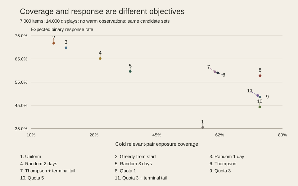
In the 7,000-item base condition, a one-observation quota increases cold relevant-pair coverage from 61.96% under Thompson sampling to 73.76%. Expected response falls from 59.03% to 57.79%. A three-observation quota with a terminal tail produces 73.13% coverage but reduces response to 49.26%.
The trade-offs change with the budget and feedback delay. The one-observation quota improves both measures against Thompson in some conditions. Greedy from start reaches 71.71% response while covering 16.31% of cold relevant pairs. Short random-then-greedy schedules also produce high response rates with much narrower coverage.
In the continuation conditions, adding a greedy window before event close reduces post-event response against a control with the same final tail. The immediate gain still raises combined response over the equally weighted event and continuation.
The practical question is what another observation can change before the objective horizon. A count target makes coverage measurable; its value depends on the decisions that remain.
1. What the public documentation establishes
Steam Next Fest has a clear public purpose: help players find upcoming games and let developers reach potential audiences. The October 2026 edition starts at 10:00 AM PDT on 19 October and ends at the same time on 26 October.[1][2]
Steam says that the first few days are randomised except for explicitly named lists and personalised segments. It then describes personalised carousels for logged-in users, using behaviour observed during the event. Categories and Steam tags also affect where games appear.[1]
This describes a transition in some discovery surfaces. The fraction of impressions allocated to exploration remains unspecified, along with the role of existing player histories in individual rankings. Internal candidate generation and ranking objectives are also undisclosed.
The distinction matters when constructing a baseline. A simulator that randomises every recommendation for two days and then becomes greedy is an experimental policy with its own assumptions.
1.1 Catalogue totals are not assignment logs
Output Lag's launch article reports 7,131 demos. Its embedded counter showed 7,288 when checked on 22 October. The methodology identifies this as its own count rather than Valve's. It measures concurrent players, checking active demos hourly and the whole festival every four hours.[3]
Those figures give a reason to examine several-thousand-item catalogues. They provide no estimate of recommendation impressions. Changes to a live counter also cannot establish historical catalogue growth.
The public demo viewer provides another useful catalogue reference, but its README warns that some demos may not officially participate in Next Fest. Its classifications describe AI use during development; this study does not use them as game-quality or preference labels.[4]
Press Preview adds a separate counting difference. Valve says it includes registered games regardless of whether their demos are live. Appearance during the event requires a released demo.[1] A press-preview entry count and a live-demo count should therefore not be presented as competing measurements of the same population.
1.2 The event can end before the value of learning ends
Valve allows demos to launch before Next Fest. It also encourages developers to consider leaving them available afterwards.[1]
A recommendation made late in the week can therefore generate information that remains useful outside the festival. The model needs to state whether it values that information.
The study therefore reports an event-only objective alongside separate continuation conditions. Both are explicit modelling choices.
2. There are two deadlines to specify
An event has an availability window. A learning system has an objective horizon: the last future decision for which information has value.
For an event-only model, the objective can be written as:
J_event(policy) = expected sum of responses to event displays
A model that also values later recommendations can instead use:
J_extended(policy) =
    expected responses during the event
    + weight * expected responses during a declared continuation
The continuation experiments use equal weight per display and the same attention rate for another seven days. These assumptions define the comparison; later Steam traffic could follow a different pattern.
Feedback timing creates a second constraint within either objective.
An action selected in batch b receives feedback at b + 1 + d.
Let the final decision batch have index H - 1. When
b + 1 + d >= H, the outcome cannot inform another decision in the
objective window.
For a model concerned only with additive responses, with no effect on future candidate availability, that action has no remaining learning benefit inside the window. Choosing the highest expected immediate response is then appropriate if the decision beliefs are valid.
The argument applies to the terminal tail of the chosen objective. An earlier stopping rule would also need to account for the decisions that feedback could still improve. The simulation uses imperfect Beta beliefs, so the policy ordering still needs to be measured.
3. The underlying ideas already have substantial prior art
Exploration under deadlines is established research.
Traca, Rudin and Yan study mortal bandits, where items appear and disappear. Their life-regulated algorithms reduce exploration of arms near disappearance. The paper includes regret analysis and experiments using randomly logged Yahoo news recommendations.[5]
This is close prior art for accounting for remaining item life. It also shows why a festival deadline needs care: a game may remain available and useful to recommend after the event.
Wang and colleagues address item-centric exploration for cold starts. Their method places a filter after an existing ranking stage. It compares predicted user satisfaction with an item's Beta posterior satisfaction rate, avoiding audience assignments predicted to be substantially worse than that item's average. They report an online short-video evaluation.[6]
The count quotas below omit that ranking model and audience-quality test. They evaluate a simpler scheduling rule.
Zhang and colleagues address delayed long-term outcomes through progressive feedback. Their impatient-bandit method combines Thompson sampling with a Bayesian filter that uses earlier observations while preserving uncertainty about later outcomes. Their application concerns podcast engagement over 60 days.[7]
The study here models delayed binary feedback without early signals. It measures the effects of that delay, leaving the filter and its production results outside the comparison.
Thompson sampling itself is a standard baseline. In the Beta-Bernoulli case, an algorithm samples plausible response probabilities from its current beliefs. It chooses the largest draw and updates the selected pair when its response arrives.[8]
The contribution is an applied comparison under explicit constraints. The policies use established ideas. The focused source review makes no exhaustive novelty claim about discovery benchmarks.
4. Evidence debt needs a unit
An under-observed game may deserve further investigation. To judge whether another display is worthwhile, a scheduler needs more than a count of missing observations.
Consider a count-based target:
D(c, i, t) = max(0, m - n(c, i, t))
Here n(c, i, t) counts delivered observations for item i in audience
c. The chosen floor m has an explicit unit: observations of that
audience-item pair.
The result is a coverage deficit relative to the chosen floor. Using it as an evidence requirement would need validation for a particular decision.
Three observations can contain three failures or three successes. Observations from a different audience may say little about a niche game's intended audience. A working model can have many observations and still be confidently wrong about another population.
Pending responses introduce another distinction. They consume attention before they become evidence. A scheduler that ignores them can allocate the same nominal deficit repeatedly while waiting for feedback.
The quota policies reserve pending allocations when deciding what to show. The reported floor coverage counts only observations delivered by the deadline. A scheduled display can therefore satisfy a reservation while its outcome remains unavailable.
4.1 Some count targets are impossible before a policy is chosen
Suppose there are K target audience-item pairs, no existing observations
and M displays. One display produces at most one observation.
The fraction of target pairs receiving at least m observations is bounded by:
count-floor coverage <= min(K, floor(M / m)) / K
With 14,000 displays and a three-observation floor:
| Items, with one target pair each | Displays per item | Maximum floor coverage |
|---|---|---|
| 1,000 | 14.00 | 100.00% |
| 3,000 | 4.67 | 100.00% |
| 7,000 | 2.00 | 66.66% |
| 15,000 | 0.93 | 31.11% |
These are optimistic upper bounds. Wrong-audience displays and late responses can reduce achievable coverage. Candidate eligibility can prevent some allocations entirely.
For independent uniform draws over items, the expected fraction never
shown is (1 - 1 / K)^M. That is approximately 13.53% at 7,000 items and
39.32% at 15,000 items for 14,000 draws.
This calculation assumes uniform catalogue sampling. The simulation below uses audience-targeted candidates. The bound shows why an exploration duration alone is insufficient to guarantee coverage: the number of available displays matters too.
Meeting the floor for every item may be a poor use of attention even when it is feasible. The product objective needs to justify the likely effect of those observations on future decisions.
5. A reproducible decision-model study
The study asks two questions. How do the declared policies trade expected response against exposure of relevant cold pairs? Does the answer change when feedback or the objective extends beyond the event?
5.1 The synthetic world
Every item has one latent favourable audience among six. Its probability
of a positive response in that audience comes from Beta(2, 2). Other
audience probabilities come from Beta(1, 19).
The two distributions create differences in audience fit. A positive binary response is a synthetic outcome, with no calibrated relationship to wishlists or player satisfaction.
| Component | Base condition |
|---|---|
| Event | 28 batches, representing four batches per day for seven days |
| Attention | 14,000 synthetic display opportunities |
| Catalogue | 7,000 items; separate size conditions use 1,000, 3,000 and 15,000 |
| Audience demand shares | 40%, 25%, 15%, 10%, 6% and 4% |
| Item audience distribution | Uniform over the six latent favourable audiences |
| Observed audience label | Correct with probability 0.85; otherwise one of the other five audiences |
| Candidate opportunities | 48 distinct matching-label items plus 16 other distinct catalogue items per request |
| Decision beliefs | Separate Beta beliefs for each audience-item pair |
| Prior mean | 0.4 for a matching observed label; 0.1 otherwise |
| Prior concentration | 2, with a separate concentration-20 condition |
| Feedback | Available at the next batch boundary, plus any declared extra delay |
The additional 16 candidates exclude the first 48, but can also carry a matching label. Every policy receives the same candidate set for each request in a world.
The random baseline therefore already benefits from coarse audience targeting. All policies allocate attention within the same retrieved opportunities.
The working Beta beliefs are misspecified for the hidden audience-mixture generator. Changing label accuracy affects candidate quality as well as the accuracy of the fixed prior means. The metadata conditions vary both mechanisms together.
The policies also learn each pair independently, without transfer between similar games.
5.2 Policies
| Policy | Decision rule |
|---|---|
| Uniform | Choose randomly within each request's candidate set |
| Greedy from start | Choose the highest posterior mean from the first batch |
| Random 1 day | Random selection for one day, then highest posterior mean |
| Random 2 days | Random selection for two days, then highest posterior mean |
| Random 3 days | Random selection for three days, then highest posterior mean |
| Thompson | Sample each candidate pair's Beta belief and choose the largest |
| Thompson + terminal tail | Thompson until feedback cannot inform another decision inside the objective; then highest mean |
| Quota 1 | Prefer a matching-label pair below a count of one; otherwise Thompson |
| Quota 3 | The same rule with a count of three |
| Quota 5 | The same rule with a count of five |
| Quota 3 + terminal tail | Quota 3 with the same terminal-tail gate |
The random-then-greedy policies continue updating means after the switch, unlike an explore-then-commit policy with frozen estimates.
Greedy selection can still expose unfamiliar pairs when candidate sets change or means tie. It has no deliberate exploration bonus, although it can learn from that incidental exposure.
When several matching-label pairs are below a quota, the quota policy chooses among those with the lowest count, breaking ties with Thompson draws. That count includes delivered observations and pending display reservations, including allocations earlier in the current batch.
Testing counts of one, three and five checks sensitivity to the chosen floor. The rule treats each missing count equally, irrespective of its potential information gain.
The candidate oracle, retained in the raw results, knows the true response probabilities and selects the best of each request's candidates. This evaluator-only information provides an upper reference for the policies, which learn from delivered outcomes.
5.3 Measures
Expected response is the average latent response probability of selected items. Using this evaluator-only quantity reduces the noise from sampled binary outcomes. The raw results also preserve the actual sampled responses used for learning.
Cold relevant-pair coverage considers only items with no pre-event observations in any audience. Among those items, it is the fraction of audience-item pairs with response probability at least 0.5 that receive an event display. Pairs on warm items are excluded even if the pair itself has no observations. This measures exposure in the synthetic population.
Delivered floor coverage is the fraction of items whose observed-label pair has at least three delivered observations by event close. It is reported for every policy, irrespective of that policy's quota.
The raw results also include item coverage and the display share of the most-exposed 1% of items. Late-feedback fraction counts event responses not yet delivered at close. An outcome delivered exactly at close counts as received, although it cannot affect another event recommendation.
5.4 Paired worlds and sensitivity conditions
There are 32 independent world seeds per condition. Within a world, policies share latent response probabilities and candidate opportunities. They also share exogenous outcome draws. Only the outcome of the selected item is delivered to a policy.
The protocol specifies 16 conditions. Four vary catalogue size while holding event attention at 14,000. Two additional conditions keep attention at two displays per item for the smallest and largest catalogues.
Other conditions add one or three days of extra feedback delay. Warm conditions provide existing observations for 20% or 60% of items. Metadata accuracy varies separately. There is also an equal-demand audience condition and a stronger-prior condition.
Warm items are chosen independently of quality. Each receives 12 pre-event observations, allocated according to audience demand. Those observations are available to all policies and are outside the event budget. The warm conditions test access to prior evidence; they omit fan-driven traffic.
Two continuation conditions retain the same items and response probabilities for another seven days at the same attention rate. One has no extra feedback delay; the other adds one day. Each includes an extra control that applies a terminal tail at the event boundary as well as at the actual end.
The complete study has 512 synthetic worlds and 5,696 policy runs. Reported 95% intervals use 10,000 bootstrap resamples of world seeds. Differences preserve seed pairing.
The intervals describe Monte Carlo uncertainty within the model. Uncertainty about the model's suitability for Steam remains outside them. The comparisons are exploratory, with no multiple-comparison significance claims.
The initial ten-policy protocol was saved before the first experiment. After its results showed strong random-then-greedy performance, a protocol amendment added the missing greedy-from-start control. Every condition and policy was rerun. World seeds and the original policy parameters were unchanged.
Both protocol hashes are retained. The protocol was locked locally; the experiment was not publicly preregistered.
6. Results under a fixed attention budget
6.1 Quotas increase coverage in the base condition
The base condition has 7,000 items and 14,000 event displays. Feedback arrives at the next batch boundary, with no extra delay. All items begin without observations.
Values below are means across 32 worlds. The coverage percentages describe the defined populations, rather than confidence levels.
| Policy | Expected response, % | Cold relevant-pair coverage, % | Delivered three-observation floor, % |
|---|---|---|---|
| Uniform | 35.53 | 57.79 | 23.64 |
| Greedy from start | 71.71 | 16.31 | 7.72 |
| Random 1 day | 69.80 | 19.73 | 8.56 |
| Random 2 days | 65.16 | 29.25 | 10.58 |
| Random 3 days | 59.61 | 37.62 | 12.97 |
| Thompson | 59.03 | 61.96 | 18.37 |
| Thompson + terminal tail | 59.50 | 61.18 | 18.10 |
| Quota 1 | 57.79 | 73.76 | 16.10 |
| Quota 3 | 48.57 | 73.73 | 32.38 |
| Quota 5 | 44.29 | 73.68 | 32.38 |
| Quota 3 + terminal tail | 49.26 | 73.13 | 32.78 |
The one-observation quota raises cold relevant-pair coverage by 11.80 percentage points against Thompson, at a response cost of 1.24 points. Increasing the quota to five produces a similar coverage mean while reducing response further.
Quota 3 + terminal tail reaches the delivered three-observation floor for 32.78% of items, compared with 18.37% for Thompson. Its expected response is 9.77 percentage points lower.
Paired differences against Thompson are:
| Policy compared with Thompson | Response difference, percentage points | Cold-coverage difference, percentage points |
|---|---|---|
| Random 1 day | +10.78 [10.58, 10.98] | -42.23 [-42.58, -41.87] |
| Quota 1 | -1.24 [-1.38, -1.09] | +11.80 [11.59, 12.02] |
| Quota 3 + terminal tail | -9.77 [-9.98, -9.56] | +11.17 [10.97, 11.36] |
Brackets contain 95% bootstrap intervals over paired world seeds.
6.2 Greedy has the highest response in the base condition
Greedy from start produces 71.71% response, with 16.31% cold relevant-pair coverage. Against Thompson, the paired response difference is +12.68 points [12.45, 12.91]. Its coverage difference is -45.65 points [-46.01, -45.29]. The most-exposed 1% receive 47.73% of displays.
Random 1 day produces a 69.80% response rate, compared with 59.03% for continuous Thompson sampling. Its cold relevant-pair coverage is much lower: 19.73% against 61.96%.
The exposure distribution also changes. The most-exposed 1% of items receive 42.63% of displays under Random 1 day, compared with 17.47% under Thompson. This describes how much attention goes to a small set of items.
The model supplies audience-targeted candidates and informative prior means before a policy acts. Greedy can then encounter unfamiliar items through changing candidate sets. Those information sources are already present in the greedy baseline.
With 60% warm items, greedy response reaches 81.60%, while cold relevant-pair coverage falls to 0.05%. Warm observations were allocated independently of item quality, so this condition leaves the effects of an established fan audience untested.
Choosing between these allocations requires a product objective. Expected response and cold discovery can support different choices.
6.3 Response stays similar at a fixed attention ratio
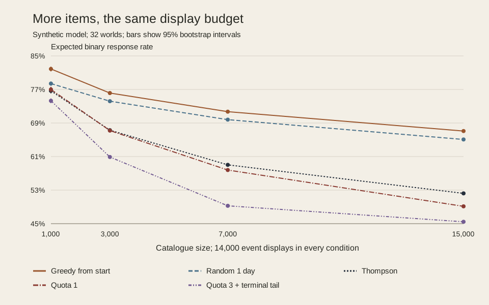
With event attention fixed at 14,000, all selected policies' response rates fall as the catalogue grows.
| Items | Greedy from start, % | Random 1 day, % | Thompson, % | Quota 1, % | Quota 3 + terminal tail, % |
|---|---|---|---|---|---|
| 1,000 | 81.89 | 78.41 | 76.68 | 77.00 | 74.30 |
| 3,000 | 76.15 | 74.20 | 67.29 | 67.20 | 60.90 |
| 7,000 | 71.71 | 69.80 | 59.03 | 57.79 | 49.26 |
| 15,000 | 67.09 | 65.08 | 52.22 | 49.13 | 45.45 |
The one-day random schedule remains above Quota 3 + terminal tail on response at every tested size. Increasing the catalogue alone produces no crossover between those two policies in this range.
Holding attention at two displays per item produces a different comparison:
| Items | Event displays | Thompson response, % | Thompson cold relevant-pair coverage, % |
|---|---|---|---|
| 1,000 | 2,000 | 59.29 | 61.10 |
| 7,000 | 14,000 | 59.03 | 61.96 |
| 15,000 | 30,000 | 59.05 | 61.82 |
The response means are similar despite a fifteen-fold difference in catalogue size. In this model, attention per item accounts for much of the earlier size effect. The experiment holds that ratio fixed; it provides no estimate of how real attention scales.
There are also positive quota results. At 1,000 items and 14,000 displays, Quota 1 exceeds Thompson by 0.33 response points, with a paired 95% interval of [0.11, 0.54]. Cold coverage improves by 0.68 points [0.51, 0.87]. At 3,000 items its response difference is -0.09 points [-0.26, 0.09], while coverage improves by 8.35 points [8.05, 8.64].
The interval at 3,000 items includes a response loss as well as a gain. A non-inferiority claim would need a justified acceptable loss and an evaluation designed around it.
7. Feedback and continuation change the decision
7.1 A terminal tail changes the cost of delayed feedback
In the base condition, replacing Thompson sampling with posterior means in the final batch increases response by 0.48 percentage points [0.47, 0.49]. Cold relevant-pair coverage falls by 0.78 points [-0.83, -0.73].
One or three days of extra delay make the terminal tail longer. They also leave 14.29% or 42.86% of event responses undelivered at close, respectively. Every policy has the same late fraction because request times and the fixed delay are shared.
The following differences are against Thompson within each condition. Brackets contain paired 95% intervals.
| Condition | Terminal-tail response difference, points | Quota 1 response difference, points | Quota 3 + tail response difference, points |
|---|---|---|---|
| Base | +0.48 [0.47, 0.49] | -1.24 [-1.38, -1.09] | -9.77 [-9.98, -9.56] |
| One day extra delay | +2.43 [2.38, 2.48] | +0.24 [0.13, 0.36] | -3.28 [-3.43, -3.13] |
| Three days extra delay | +6.55 [6.38, 6.70] | +0.63 [0.54, 0.72] | +4.18 [4.08, 4.30] |
| 20% warm items | +0.46 [0.45, 0.48] | -1.48 [-1.61, -1.35] | -9.98 [-10.13, -9.83] |
| 60% warm items | +0.40 [0.39, 0.41] | -1.66 [-1.78, -1.54] | -8.89 [-9.03, -8.76] |
| Uninformative labels | +0.87 [0.85, 0.90] | -0.62 [-0.78, -0.46] | -10.77 [-11.06, -10.49] |
| Perfect labels | +0.44 [0.43, 0.45] | -1.16 [-1.30, -1.02] | -7.50 [-7.64, -7.37] |
| Equal audience demand | +0.57 [0.55, 0.58] | -2.03 [-2.16, -1.89] | -10.76 [-10.89, -10.62] |
| Prior concentration 20 | +0.43 [0.42, 0.45] | -2.23 [-2.41, -2.05] | -7.75 [-7.94, -7.56] |
Zero extra delay still includes the batch boundary. One day of extra delay means feedback arrives five six-hour batches after a display.
The delayed quota results also require both outcome measures. Quota 1 improves cold coverage against Thompson by 12.04 points with one day of extra delay and 12.05 points with three days. In those conditions its response difference is positive too.
Quota 3 + terminal tail improves response against Thompson under three days of extra delay, but cold coverage falls by 1.20 points [-1.42, -0.97]. The tail-only control has a larger response gain of 6.55 points, with lower coverage. An improvement against a horizon-unaware reference does not establish that the count quota caused the response benefit.
The quota policies also count pending reservations, while ordinary Thompson samples its delivered-data beliefs without such reservations. These delayed comparisons do not isolate a quota's effect from pending-work scheduling.
7.2 The event-tail window has a post-event cost
When the same items remain useful for another seven days, the actual objective horizon moves. The end-only terminal-tail policy therefore matches ordinary Thompson during the event and becomes greedy only near the later end.
The extra control inserts a greedy window before event close, then resumes Thompson afterwards. Both controls use the same tail at the actual end. Comparing them isolates the added event boundary.
| Extra delay | Policy | Event response, % | Post-event response, % | Combined response, % |
|---|---|---|---|---|
| None | Greedy from start | 71.71 | 79.05 | 75.38 |
| None | Random 1 day | 69.80 | 80.31 | 75.06 |
| None | Thompson | 59.03 | 73.51 | 66.27 |
| None | End-only terminal tail | 59.03 | 73.89 | 66.46 |
| None | Event and end tails | 59.50 | 73.67 | 66.59 |
| One day | Greedy from start | 67.76 | 81.74 | 74.75 |
| One day | Random 1 day | 65.99 | 81.26 | 73.62 |
| One day | Thompson | 54.59 | 72.21 | 63.40 |
| One day | End-only terminal tail | 54.59 | 74.11 | 64.35 |
| One day | Event and end tails | 57.02 | 73.18 | 65.10 |
Against the matched end-only-tail control, the extra event window reduces post-event response by 0.22 percentage points, with a paired 95% interval of [-0.34, -0.12]. With one day of extra delay, the reduction is 0.93 points [-1.04, -0.81]. Those comparisons show a later cost from the earlier change in exploration.
The immediate gains outweigh that cost over the tested continuation. Combined response rises by 0.13 points [0.07, 0.18] without extra delay and 0.75 points [0.69, 0.81] with one day of extra delay. These results use equal weight per display for the event and the following seven days.
The paired control comparison was added during manuscript QA using the existing runs. Comparing only with ordinary Thompson would also change behaviour at the final boundary and obscure the post-event cost.
Thompson is not an optimal finite-horizon policy. New observations can have some future value while still costing more than they return. The terminal-tail argument identifies when feedback has no remaining use inside the objective; it leaves the earlier schedule open.
8. What a platform evaluation would need
Public popularity charts cannot supply the missing counterfactuals. A demo with few concurrent players may have had few displays. It may have received poorly matched displays, or players may have tried it and left. The same count can be consistent with different mechanisms.
Li and colleagues' offline contextual-bandit work makes the partial-label problem explicit. Outcomes are observed for the actions taken by a logging policy, not every action a new policy might choose. Their replay evaluator uses random logging under stated assumptions to obtain an unbiased evaluation. They also discuss the modelling bias introduced by simulators.[9]
A credible empirical follow-up would need a platform experiment or appropriate assignment logs. Each record should identify the discovery surface and eligible candidates, along with the chosen item and its assignment probability. The evaluation needs a defined response outcome and separate timestamps for display and feedback ingestion.
Existing audience evidence needs a defined cut-off. An algorithm cannot be evaluated as cold-start if it receives future observations or private labels unavailable to its comparator.
For a real player study, the outcome would need to be grounded in the experience of trying a demo. A tile click can be an early signal. Using it as a surrogate for later satisfaction needs separate validation.
The experiment would also need to define its trade-off. A minimum acceptable player outcome can be a guardrail while discovery coverage is examined separately. Equal exposure is a different policy objective and should be justified as such.
Collection of player-level records would require appropriate privacy controls. Nothing in this paper calls for scraping private developer dashboards or assembling identities across public services.
The earlier game-discovery paper asks whether claims about a game carry adequate source and scope information.[10] Better descriptive evidence may improve retrieval. Attention allocation still needs its own evaluation.
9. The strongest counterargument
This model may be too simple to select a production policy.
Real recommendation systems can transfer information across related items. They have richer player histories, and candidate retrieval can adapt as evidence changes. A game can appeal to several audiences. Playing a demo also consumes a different amount of time from seeing a tile.
The study omits those mechanisms. Repeated-user fatigue is absent. Every synthetic display has the same budget cost, and responses are stationary conditional on an audience-item pair. A policy's choices do not change later demand or developer behaviour.
These assumptions are especially important for catalogue scaling. Independent pair beliefs make a new item expensive to learn about. A production system with effective transfer may need much less item-specific feedback. Conversely, a badly misspecified model can require more careful investigation than a count floor suggests.
The common candidate generator isolates allocation within the model. It also excludes a potentially decisive part of a real system. A policy cannot choose a relevant game that its retrieval stage never supplies.
The study provides conditional trade-offs and an auditable test harness. Choosing a production policy would require an evaluation that represents the omitted mechanisms and actual player outcomes.
The baseline set is also limited to recognisable policies and a few random-then-greedy schedules. More capable contextual-bandit methods remain to be compared.
10. What this paper does not claim
This paper does not establish that Steam stops exploring too early. It does not identify a hidden threshold at which a festival catalogue becomes too large.
It does not introduce deadline-sensitive exploration or reproduce the item-centric filter in the cited industry paper. The count quotas are simple controls, not a novel information-gain algorithm.
It does not measure recommendation quality, wishlist conversion or commercial success on Steam. The relevant-pair labels exist only in the synthetic evaluator.
It does not establish that reducing exposure concentration helps every player, or that every game deserves the same observation budget. It makes no claim about long-term creative diversity or developer incentives.
Conclusion
Count-based coverage targets can exceed the available observation budget before any ranking policy is chosen. The simple budget bound makes that constraint explicit.
Within the synthetic model, increasing a quota can raise delivered count coverage while reducing expected response substantially. A smaller quota improves both headline measures against Thompson in some conditions. The policy ordering changes with the available attention and feedback timing.
The continuation comparison shows why the objective matters. An extra event-tail window reduces post-event response against the matched end-only-tail control. Its immediate gains still improve combined response over the tested continuation. That ordering could change with different continuation weights or duration.
Before choosing an exploration schedule, specify which future decisions count and when feedback reaches them. A coverage target can then be judged against its cost and the opportunities left to use what it reveals.
Reproducibility
The study bundle contains the protocol, executable policies and raw results. The same files are available in the artifact directory.
The primary records are individual runs and daily checkpoints. Paired comparisons against Thompson retain uncertainty across world seeds. The matched continuation comparison isolates the extra event-tail window.
Run the focused tests, create a fresh result directory with study.py,
then run analyse.py against that directory. Exact commands and
dependencies are in the artifact README. No network access or private data
is required for the experiment.
About the author
Jason Doyle writes about reliable software systems and applied AI. He publishes at jasondoyle.ie.
References
-
Valve, Steam Next Fest, accessed 22 October 2026, https://partner.steamgames.com/doc/marketing/upcoming_events/nextfest.
-
Valve, Steam Next Fest: October 2026 Edition, accessed 22 October 2026, https://partner.steamgames.com/doc/marketing/upcoming_events/nextfest/2026october.
-
Output Lag, Steam Next Fest Live Chart, accessed 22 October 2026, https://outputlag.com/news/steam-next-fest-live-chart/.
-
SonOfSaris, Viewer for Steam Next Fest, README at commit
c272801948b81dabe951d09d3022fb894cdde80d, accessed 22 October 2026, https://github.com/SonOfSaris/ViewerForSteamNextFest/blob/c272801948b81dabe951d09d3022fb894cdde80d/README.md. -
Stefano Traca, Cynthia Rudin and Weiyu Yan, Reducing Exploration of Dying Arms in Mortal Bandits, UAI 2019, https://arxiv.org/abs/1907.02571v1.
-
Dong Wang and colleagues, Item-centric Exploration for Cold Start Problem, ACM RecSys 2025 Industry Track, https://arxiv.org/abs/2507.09423v1.
-
Kelly W. Zhang and colleagues, Impatient Bandits: Optimizing for the Long-Term Without Delay, Journal of Machine Learning Research 27(156), 2026, pp. 1-58, https://jmlr.org/papers/v27/25-0030.html.
-
Daniel Russo and colleagues, A Tutorial on Thompson Sampling, arXiv:1707.02038v3, https://arxiv.org/abs/1707.02038v3.
-
Lihong Li, Wei Chu, John Langford and Xuanhui Wang, Unbiased Offline Evaluation of Contextual-bandit-based News Article Recommendation Algorithms, arXiv:1003.5956, 2010, https://arxiv.org/abs/1003.5956.
-
Jason Doyle, Game Discovery Is an Evidence Problem, 28 September 2026, https://jasondoyle.ie/whitepapers/game-discovery-is-an-evidence-problem/.